WK Model Specifics
2020 Models
In pdrtpy, these are referred to as the wk2020 ModelSet.
These model data start with the 2006 PDR model code and add improved physics and chemistry. Critical updates include those discussed in Neufeld & Wolfire 2016, plus photo rates from Heays et al. 2017, oxygen chemistry rates from Kovalenko et al. 2018 and Tran et al. 2018, and carbon chemistry rates from Dagdigian 2019. We have also implemented new collisional excitation rates for [O I] from Lique et al. 2018 (and Lique private communication) and have included 13C chemistry along with the emitted line intensities for [13C II] and 13CO. In Box 1, we show the currently available spectral lines and those we expect to deploy later in the project. In addition, we will compute ModelSets for a full range of metallicity \(Z\).
Alternate Viewing Angle Models
The viewing angle models calculate the emitted line intensity along a line-of-sight
at angle, \(\theta\), with respect to the illuminated face of the PDR. The
angle \(\theta=0 \) is a line that is perpendicular to the face while the
angle \(\theta=90\) is a line that is parallel to the face.
The line intensity
for each transition as well as the integrated far-infrared intensity
is calculated as in Pabst et al. 2017, A&A, 606, A29. We make the
assumption that each line of sight passes through all layers of the PDR
to an optical depth of \(A_v=7\) from the face. This means that the integral
along the line-of-sight as well as \(A_v\)
increases as \(7/cos(\theta)\),
and the thickness of the PDR increases as
\(7*tan(\theta)\)
.
The user should keep in mind that this assumption may lead
to unrealistically large \(A_v\) that should be checked against observations
if possible. The different angles and \(A_v\)s are given in the FITS headers
as follows:
- LOSANGLE – angle in degrees with respect to illuminated face of PDR
- AV – optical depth in magnitudes of visual extinction of PDR along a line through the illuminated face to the deepest layers. All models are fixed at \(A_v=7\).
- AVPERP – optical depth in magnitudes of visual extinction of the PDR perpendicular to \(A_v\).
- AVLOS – optical depth in magnitudes of visual extinction of the PDR along the line-of-sight.
2006 Models
In pdrtpy, these are referred to as the wk2006 ModelSet.
These models are identical to those that were available in the now-deprecated web-based PDR Toolbox. They have metallicity \(Z=1\), and contain [C I], [C II], [O I], Fe, Si, H2 lines and the 12CO ladder up to \(J=14\rightarrow 13\). For some lines, \(Z=3\) is also available.
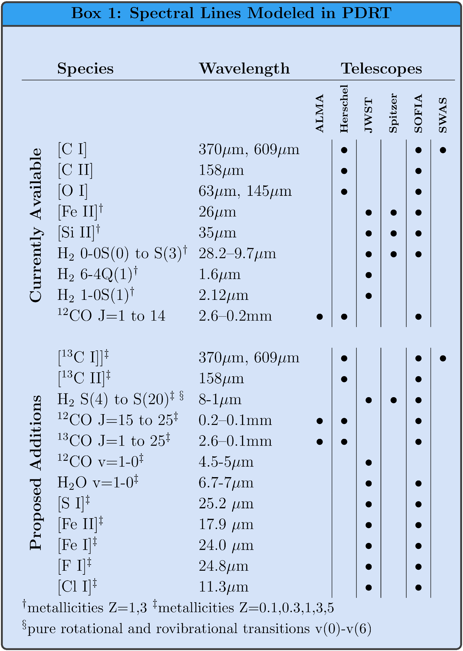
Current and future spectral line and metallicity coverage of the PDR Toolbox.
WK Model Parameters
Our 2006 models use the standard parameters from Kaufman et al. 1999. Changes for the 2020 models are listed below. The formation rate of H2 goes as \(R_{form}~n_{HI}~n\). The PAH abundance \(X_{PAH}=n_{PAH}/n\).
| Parameter | Symbol | Value |
|---|---|---|
| Turbulent Doppler velocity | \(\delta v_D\) | 1.5 km s-1 |
| Carbon abundance | \(X_C\) | \(1.4\times10^{-4}\) |
| Oxygen abundance | \(X_O\) | \(3.0\times10^{-4}\) |
| Silicon abundance | \(X_{Si}\) | \(1.7\times10^{-6}\) |
| Sulfur abundance | \(X_{S}\) | \(2.8\times10^{-5}\) |
| Iron abundance | \(X_{Fe}\) | \(1.7\times10^{-7}\) |
| Magnesium abundance | \(X_{Mg}\) | \(1.1\times10^{-6}\) |
| Dust abundance relative to diffuse ISM | \(\delta_d\) | 1 |
| FUV dust absorption/visual extinction | \(\delta_{UV}\) | 1.8 |
| Dust visual extinction per H | \(\sigma_V\) | \(5\times10^{-22}\) cm-2 |
| Formation rate of H2 on dust | \(R_{form}\) | \(3\times10^{-17}\) s-1 |
| PAH abundance | \(X_{PAH}\) | \(5\times10^{-7}\) |
| Cloud H density | \(n\) | \(10^{1} - 10^{7}\) cm-3 |
| Incident UV flux | \(G_0\) | \(10^{-0.5} - 10^{6.5}\) Habing |
| Parameter | Symbol | Value |
|---|---|---|
| Carbon abundance | \(X_C\) | \(1.6\times10^{-4}\) |
| Oxygen abundance | \(X_O\) | \(3.2\times10^{-4}\) |
| Dust visual extinction per H | \(\sigma_V\) | \(5.26\times10^{-22}\) cm-2 |
| Formation rate of H2 on dust | \(R_{form}\) | \(6\times10^{-17}\) s-1 |
| PAH abundance | \(X_{PAH}\) | \(2\times10^{-7}\) |
| Viewing Angle | \(i_{LOS}\) | 0 (face-on) to 75 degrees |